Activation Functions
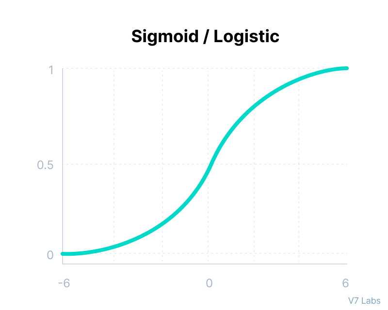
Sigmoid / Logistic Function

import math;

def sigmoid(x):
  return 1 / (1 + math.exp(-x))
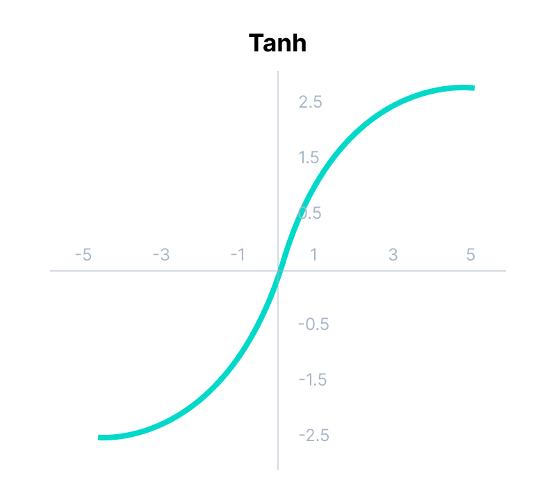
tanh Function

import math;

def tanh(x):
  return (math.exp(x) - math.exp(-x)) / (math.exp(x) + math.exp(-x))
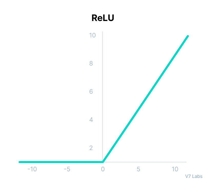
ReLU

import math;

def relu(x):
    return max(0,x)
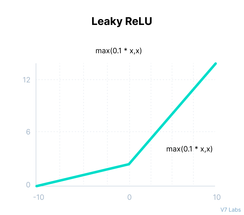
Leaky ReLU

import math;

def leaky_relu(x):
    return max(0.1*x,x)
Loss \ Cost Functions
Mean Absolute Error/L1 Loss (Regression Losses)
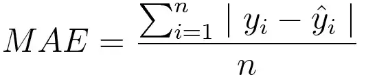
Mean absolute error, on the other hand, is measured as the average sum of absolute differences between predictions and actual observations. Like MSE, this as well measures the magnitude of error without considering their direction. Unlike MSE, MAE needs more complicated tools such as linear programming to compute the gradients. Plus MAE is more robust to outliers since it does not make use of squares.
# Plain implementation

import numpy as np
y_hat = np.array([0.000, 0.166, 0.333])
y_true = np.array([0.000, 0.254, 0.998])

print("d is: " + str(["%.8f" % elem for elem in y_hat]))
print("p is: " + str(["%.8f" % elem for elem in y_true]))

def mae(predictions, targets):
    total_error = 0
    for yp, yt in zip(predictions, targets):
        total_error += abs(yp - yt)
    print("Total error is:",total_error)
    mae = total_error/len(predictions)
    print("Mean absolute error is:",mae)
    return mae

# Usage : mae(predictions, targets)
# Implementation using numpy
import numpy as np
y_hat = np.array([0.000, 0.166, 0.333])
y_true = np.array([0.000, 0.254, 0.998])

print("d is: " + str(["%.8f" % elem for elem in y_hat]))
print("p is: " + str(["%.8f" % elem for elem in y_true]))

def mae_np(predictions, targets):
    return np.mean(np.abs(predictions-targets))

mae_val = mae_np(y_hat, y_true)
print ("mae error is: " + str(mae_val))
Mean Square Error/Quadratic Loss/L2 Loss (Regression Losses)
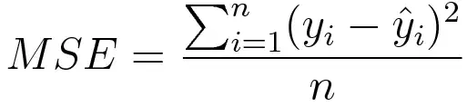
Mean square error is measured as the average of the squared difference between predictions and actual observations. It’s only concerned with the average magnitude of error irrespective of their direction. However, due to squaring, predictions that are far away from actual values are penalized heavily in comparison to less deviated predictions. Plus MSE has nice mathematical properties which make it easier to calculate gradients.
# Plain implementation

import numpy as np

y_hat = np.array([0.000, 0.166, 0.333])
y_true = np.array([0.000, 0.254, 0.998])

def rmse(predictions, targets):
    total_error = 0
    for yt, yp in zip(targets, predictions):
        total_error += (yt-yp)**2
    print("Total Squared Error:",total_error)
    mse = total_error/len(y_true)
    print("Mean Squared Error:",mse)
    return mse

print("d is: " + str(["%.8f" % elem for elem in y_hat]))
print("p is: " + str(["%.8f" % elem for elem in y_true]))

rmse_val = rmse(y_hat, y_true)
print("rms error is: " + str(rmse_val))
# Implementation using numpy

import numpy as np

y_hat = np.array([0.000, 0.166, 0.333])
y_true = np.array([0.000, 0.254, 0.998])

def rmse(predictions, targets):
    return np.mean(np.square(targets-predictions))

print("d is: " + str(["%.8f" % elem for elem in y_hat]))
print("p is: " + str(["%.8f" % elem for elem in y_true]))

rmse_val = rmse(y_hat, y_true)
print("rms error is: " + str(rmse_val))
Log Loss or Binary Cross Entropy

import numpy as np

y_predicted = np.array([[0.25,0.25,0.25,0.25],[0.01,0.01,0.01,0.96]])
y_true = np.array([[0,0,0,1],[0,0,0,1]])

def cross_entropy(predictions, targets, epsilon=1e-10):
    predictions = np.clip(predictions, epsilon, 1. - epsilon)
    N = predictions.shape[0]
    ce_loss = -np.sum(np.sum(targets * np.log(predictions + 1e-5)))/N
    return ce_loss
cross_entropy_loss = cross_entropy(predictions, targets)
print ("Cross entropy loss is: " + str(cross_entropy_loss))

# OR

def log_loss(predictions, targets, epsilon=1e-10):
    predicted_new = [max(i,epsilon) for i in predictions]
    predicted_new = [min(i,1-epsilon) for i in predicted_new]
    predicted_new = np.array(predicted_new)
    return -np.mean(targets*np.log(predicted_new)+(1-y_true)*np.log(1-predicted_new))
For more functions refer ‘Common Loss functions in machine learning’ By Ravindra Parmar
Gradient Descent
Gradient Descent
# Single Feature
import numpy as np
import matplotlib.pyplot as plt

%matplotlib inline

def gradient_descent(x, y, epochs = 10000, loss_thresold = 0.5, rate = 0.01):
    w1 = bias = 0
    n = len(x)
    plt.scatter(x, y, color='red', marker='+', linewidth='5')
    for i in range(epochs):
        y_predicted = (w1 * x)+ bias
        plt.plot(x, y_predicted, color='green')
        md = -(2/n)*sum(x*(y-y_predicted))
        yd = -(2/n)*sum(y-y_predicted)
        w1 = w1 - rate * md
        bias = bias - rate * yd
        print ("m {}, b {}, cost {} iteration {}".format(m_curr,b_curr,cost, i))

# Usage
x = np.array([1,2,3,4,5])
y = np.array([5,7,9,11,13])
gradient_descent(x, y, 500)

---

# Multiple Feature
def gradient_descent(x1, x2, y, epochs = 10000, loss_thresold = 0.5, rate = 0.01):
    w1 = w2 = bias = 1
    rate = 0.5
    n = len(x1)
    for i in range(epochs):
        weighted_sum = (w1 * x1) + (w2 * x2) + bias
        y_predicted = sigmoid_numpy(weighted_sum)
        loss = log_loss(y_predicted, y)

        w1d = (1/n)*np.dot(np.transpose(x1),(y_predicted-y))
        w2d = (1/n)*np.dot(np.transpose(x2),(y_predicted-y))

        bias_d = np.mean(y_predicted-y)
        w1 = w1 - rate * w1d
        w2 = w2 - rate * w2d
        bias = bias - rate * bias_d

        print (f'Epoch:{i}, w1:{w1}, w2:{w2}, bias:{bias}, loss:{loss}')

        if loss<=loss_thresold:
            break

    return w1, w2, bias

# Usage
gradient_descent(
    X_train_scaled['age'],
    X_train_scaled['affordibility'],
    y_train,
    1000,
    0.4631
)
# custom neural network class

class myNN:

    def __init__(self):
        self.w1 = 1
        self.w2 = 1
        self.bias = 0

    def sigmoid_numpy(self, X):
        import numpy as np;
        return 1/(1+np.exp(-X))

    def log_loss(self, y_true, y_predicted):
        import numpy as np;
        epsilon = 1e-15
        y_predicted_new = [max(i,epsilon) for i in y_predicted]
        y_predicted_new = [min(i,1-epsilon) for i in y_predicted_new]
        y_predicted_new = np.array(y_predicted_new)
        return -np.mean(y_true*np.log(y_predicted_new)+(1-y_true)*np.log(1-y_predicted_new))

    def fit(self, X, y, epochs, loss_thresold):
        self.w1, self.w2, self.bias = self.gradient_descent(X['age'],X['affordibility'],y, epochs, loss_thresold)
        print(f"Final weights and bias: w1: {self.w1}, w2: {self.w2}, bias: {self.bias}")

    def predict(self, X_test):
        weighted_sum = self.w1*X_test['age'] + self.w2*X_test['affordibility'] + self.bias
        return self.sigmoid_numpy(weighted_sum)

    def gradient_descent(self, age,affordability, y_true, epochs, loss_thresold):
        import numpy as np;
        w1 = w2 = 1
        bias = 0
        rate = 0.5
        n = len(age)
        for i in range(epochs):
            weighted_sum = w1 * age + w2 * affordability + bias
            y_predicted = self.sigmoid_numpy(weighted_sum)
            loss = self.log_loss.log_loss(y_true, y_predicted)

            w1d = (1/n)*np.dot(np.transpose(age),(y_predicted-y_true))
            w2d = (1/n)*np.dot(np.transpose(affordability),(y_predicted-y_true))

            bias_d = np.mean(y_predicted-y_true)
            w1 = w1 - rate * w1d
            w2 = w2 - rate * w2d
            bias = bias - rate * bias_d

            if i%50==0:
                print (f'Epoch:{i}, w1:{w1}, w2:{w2}, bias:{bias}, loss:{loss}')

            if loss<=loss_thresold:
                print (f'Epoch:{i}, w1:{w1}, w2:{w2}, bias:{bias}, loss:{loss}')
                break

        return w1, w2, bias


# Usage
customModel = myNN()
customModel.fit(X_train_scaled, y_train, epochs=8000, loss_thresold=0.4631)

# Usage
customModel = myNN()
customModel.fit(
        X_train_scaled,
        y_train,
        epochs=8000,
        loss_thresold=0.4631
)
Batch Gradient Descent
def batch_gradient_descent(X, y_true, epochs, learning_rate = 0.01):

    number_of_features = X.shape[1]
    # numpy array with 1 row and columns equal to number of features. In
    # our case number_of_features = 2 (area, bedroom)
    w = np.ones(shape=(number_of_features))
    b = 0
    total_samples = X.shape[0] # number of rows in X

    cost_list = []
    epoch_list = []

    for i in range(epochs):
        y_predicted = np.dot(w, X.T) + b

        w_grad = -(2/total_samples)*(X.T.dot(y_true-y_predicted))
        b_grad = -(2/total_samples)*np.sum(y_true-y_predicted)

        w = w - learning_rate * w_grad
        b = b - learning_rate * b_grad

        cost = np.mean(np.square(y_true-y_predicted)) # MSE (Mean Squared Error)

        if i%10==0:
            cost_list.append(cost)
            epoch_list.append(i)

    return w, b, cost, cost_list, epoch_list

w, b, cost, cost_list, epoch_list = batch_gradient_descent(
    scaled_X,
    scaled_y.reshape(scaled_y.shape[0],),
    500
)
w, b, cost
Mini Batch Gradient Descent
def mini_batch_gradient_descent(X, y_true, epochs = 100, batch_size = 5, learning_rate = 0.01):

    number_of_features = X.shape[1]
    # numpy array with 1 row and columns equal to number of features. In
    # our case number_of_features = 3 (area, bedroom and age)
    w = np.ones(shape=(number_of_features))
    b = 0
    total_samples = X.shape[0] # number of rows in X

    if batch_size > total_samples: # In this case mini batch becomes same as batch gradient descent
        batch_size = total_samples

    cost_list = []
    epoch_list = []

    num_batches = int(total_samples/batch_size)

    for i in range(epochs):
        random_indices = np.random.permutation(total_samples)
        X_tmp = X[random_indices]
        y_tmp = y_true[random_indices]

        for j in range(0,total_samples,batch_size):
            Xj = X_tmp[j:j+batch_size]
            yj = y_tmp[j:j+batch_size]
            y_predicted = np.dot(w, Xj.T) + b

            w_grad = -(2/len(Xj))*(Xj.T.dot(yj-y_predicted))
            b_grad = -(2/len(Xj))*np.sum(yj-y_predicted)

            w = w - learning_rate * w_grad
            b = b - learning_rate * b_grad

            cost = np.mean(np.square(yj-y_predicted)) # MSE (Mean Squared Error)

        if i%10==0:
            cost_list.append(cost)
            epoch_list.append(i)

    return w, b, cost, cost_list, epoch_list

w, b, cost, cost_list, epoch_list = mini_batch_gradient_descent(
    scaled_X,
    scaled_y.reshape(scaled_y.shape[0],),
    epochs = 120,
    batch_size = 5
)
w, b, cost
Stochastic Gradient Descent
def stochastic_gradient_descent(X, y_true, epochs, learning_rate = 0.01):

    number_of_features = X.shape[1]
    # numpy array with 1 row and columns equal to number of features. In
    # our case number_of_features = 3 (area, bedroom and age)
    w = np.ones(shape=(number_of_features))
    b = 0
    total_samples = X.shape[0]

    cost_list = []
    epoch_list = []

    for i in range(epochs):
        random_index = random.randint(0,total_samples-1) # random index from total samples
        sample_x = X[random_index]
        sample_y = y_true[random_index]

        y_predicted = np.dot(w, sample_x.T) + b

        w_grad = -(2/total_samples)*(sample_x.T.dot(sample_y-y_predicted))
        b_grad = -(2/total_samples)*(sample_y-y_predicted)

        w = w - learning_rate * w_grad
        b = b - learning_rate * b_grad

        cost = np.square(sample_y-y_predicted)

        if i%100==0: # at every 100th iteration record the cost and epoch value
            cost_list.append(cost)
            epoch_list.append(i)

    return w, b, cost, cost_list, epoch_list

w_sgd, b_sgd, cost_sgd, cost_list_sgd, epoch_list_sgd = SGD(
    scaled_X,
    scaled_y.reshape(scaled_y.shape[0],),
    10000
)
w_sgd, b_sgd, cost_sgd