Category: Machine Learning, Deep Learning & Artificial Intelligence
Machine learning is a branch of artificial intelligence (AI) and computer science which focuses on the use of data and algorithms to imitate the way that humans learn, gradually improving its accuracy.
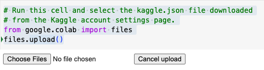
# Run this cell and select the kaggle.json file downloaded
# from the Kaggle account settings page.

from google.colab import files
files.upload()

# This will prompt the file upload control, so that we can uppload the file to the temporark work space.
# Next, install the Kaggle API client.
!pip install -q kaggle

# The Kaggle API client expects this file to be in ~/.kaggle, so move it there.
!mkdir -p ~/.kaggle
!cp kaggle.json ~/.kaggle/

# This permissions change avoids a warning on Kaggle tool startup.
!chmod 600 ~/.kaggle/kaggle.json

# Searching for dataset
!kaggle datasets list -s dogbreedidfromcomp

# Downloading dataset in the current directory
!kaggle datasets download catherinehorng/dogbreedidfromcomp

# Unzipping downloaded file and removing unusable file
!unzip dog_dataset/dogbreedidfromcomp.zip -d dog_dataset
Azure Databricks is a cloud-scale platform for data analytics and machine learning. In this course, you’ll learn how to use Azure Databricks to explore, prepare, and model data; and integrate Databricks machine learning processes with Azure Machine Learning.
This course teaches you to leverage your existing knowledge of Python and machine learning to manage data ingestion and preparation, model training and deployment, and machine learning solution monitoring with Azure Machine Learning and MLflow.
# Calculate the number of empty cells in each column
# The following line consists of three commands. Try
# to think about how they work together to calculate
# the number of missing entries per column
missing_data = dataset.isnull().sum().to_frame()

# Rename column holding the sums
missing_data = missing_data.rename(columns={0:'Empty Cells'})

# Print the results
print(missing_data)

## OR
print(dataset.isnull().sum().to_frame().rename(columns={0:'Empty Cells'}))

# Show the missing value rows
dataset[dataset.isnull().any(axis=1)]
EDA
import pandas as pd
# Load data from a text file
!wget https://raw.githubusercontent.com/MicrosoftDocs/mslearn-introduction-to-machine-learning/main/Data/ml-basics/grades.csv
df_students = pd.read_csv('grades.csv',delimiter=',',header='infer')
# Remove any rows with missing data
df_students = df_students.dropna(axis=0, how='any')
# Calculate who passed, assuming '60' is the grade needed to pass
passes = pd.Series(df_students['Grade'] >= 60)
# Save who passed to the Pandas dataframe
df_students = pd.concat([df_students, passes.rename("Pass")], axis=1)
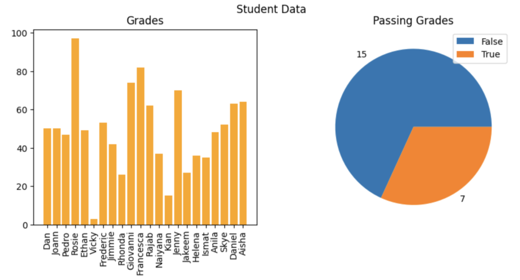
# Create a figure for 2 subplots (1 row, 2 columns)
fig, ax = plt.subplots(1, 2, figsize = (10,4))
# Create a bar plot of name vs grade on the first axis
ax[0].bar(x=df_students.Name, height=df_students.Grade, color='orange')
ax[0].set_title('Grades')
ax[0].set_xticklabels(df_students.Name, rotation=90)
# Create a pie chart of pass counts on the second axis
pass_counts = df_students['Pass'].value_counts()
ax[1].pie(pass_counts, labels=pass_counts)
ax[1].set_title('Passing Grades')
ax[1].legend(pass_counts.keys().tolist())
# Add a title to the Figure
fig.suptitle('Student Data')
# Show the figure
fig.show()
# Create a function that we can re-use
# Create a function that we can re-use
def show_distribution_with_quantile(var_data, quantile = 0):
'''
This function will make a distribution (graph) and display it
'''
if(quantile > 0){
# calculate the quantile percentile
q01 = var_data.quantile(quantile)
print(f"quantile = {q01}")
var_data = var_data[var_data>q01]
}
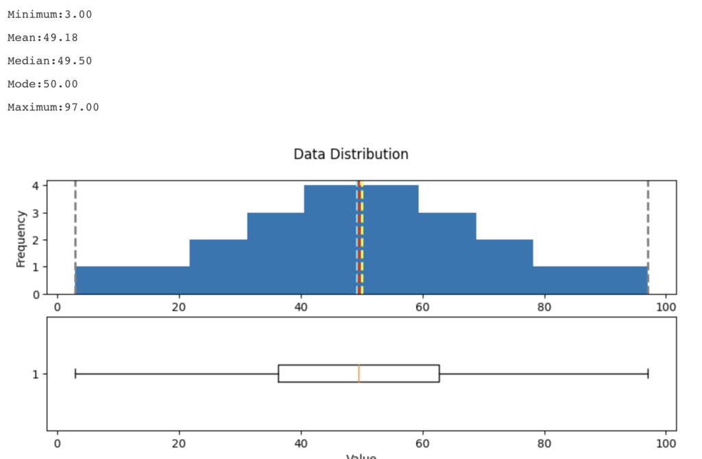
# Get statistics
min_val = var_data.min()
max_val = var_data.max()
mean_val = var_data.mean()
med_val = var_data.median()
mod_val = var_data.mode()[0]
print('Minimum:{:.2f}\nMean:{:.2f}\nMedian:{:.2f}\nMode:{:.2f}\nMaximum:{:.2f}\n'.format(min_val,
mean_val,
med_val,
mod_val,
max_val))
# Create a figure for 2 subplots (2 rows, 1 column)
fig, ax = plt.subplots(2, 1, figsize = (10,4))
# Plot the histogram
ax[0].hist(var_data)
ax[0].set_ylabel('Frequency')
# Add lines for the mean, median, and mode
ax[0].axvline(x=min_val, color = 'gray', linestyle='dashed', linewidth = 2)
ax[0].axvline(x=mean_val, color = 'cyan', linestyle='dashed', linewidth = 2)
ax[0].axvline(x=med_val, color = 'red', linestyle='dashed', linewidth = 2)
ax[0].axvline(x=mod_val, color = 'yellow', linestyle='dashed', linewidth = 2)
ax[0].axvline(x=max_val, color = 'gray', linestyle='dashed', linewidth = 2)
# Plot the boxplot
ax[1].boxplot(var_data, vert=False)
ax[1].set_xlabel('Value')
# Add a title to the Figure
fig.suptitle('Data Distribution')
# Show the figure
fig.show()
# Get the variable to examine
col = df_students['Grade']
# Call the function
show_distribution(col)
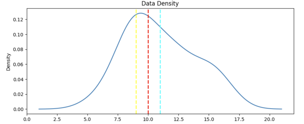
def show_density(var_data):
    fig = plt.figure(figsize=(10,4))

    # Plot density
    var_data.plot.density()

    # Add titles and labels
    plt.title('Data Density')

    # Show the mean, median, and mode
    plt.axvline(x=var_data.mean(), color = 'cyan', linestyle='dashed', linewidth = 2)
    plt.axvline(x=var_data.median(), color = 'red', linestyle='dashed', linewidth = 2)
    plt.axvline(x=var_data.mode()[0], color = 'yellow', linestyle='dashed', linewidth = 2)

    # Show the figure
    plt.show()

# Get the density of StudyHours
show_density(col)
Azure Databricks
Mount a remote Azure storage account as a DBFS folder, using the dbutils module:
data_storage_account_name = '<data_storage_account_name>'
data_storage_account_key = '<data_storage_account_key>'

data_mount_point = '/mnt/data'

data_file_path = '/bronze/wwi-factsale.csv'

dbutils.fs.mount(
  source = f"wasbs://dev@{data_storage_account_name}.blob.core.windows.net",
  mount_point = data_mount_point,
  extra_configs = {f"fs.azure.account.key.{data_storage_account_name}.blob.core.windows.net": data_storage_account_key})

display(dbutils.fs.ls("/mnt/data"))
#this path is available as dbfs:/mnt/data for spark APIs, e.g. spark.read
#this path is available as file:/dbfs/mnt/data for regular APIs, e.g. os.listdir

# %fs magic command - for accessing the dbutils filesystem module. Most dbutils.fs commands are available using %fs magic commands
We can override the cell’s default programming language by using one of the following magic commands at the start of the cell:
%python – for cells running python code
%scala– for cells running scala code
%r– for cells running R code
%sql – for cells running sql code
Additional magic commands are available:
%md – for descriptive cells using markdown
%sh– for cells running shell commands
%run – for cells running code defined in a separate notebook
%fs – for cells running code that uses dbutils commands
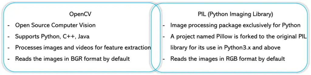
Image is simply a matrix of pixels and each pixel is a single, square-shaped point of colored light. This can be explained quickly with a grayscaled image. grayscaled image is the image where each pixel represents different shades of a gray color.
Difference between OpenCV and PIL | Image by Author
I mostly use OpenCV to complete my tasks as I find it 1.4 times quicker than PIL.
Let’s see, how the image can be processed using both — OpenCV and PIL.
Note: OpenCV images are in BGR color format, while Pillow images are in RGB color format. So we have to manually convert the color format from one to another.
Note: It is hard to get the depth/channels directly from a Pillow image object, the easier way to do this would be to first convert it to an OpenCV image (ndarray) and then get the shape.
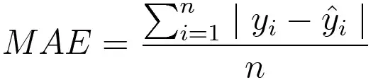
Mean absolute error, on the other hand, is measured as the average sum of absolute differences between predictions and actual observations. Like MSE, this as well measures the magnitude of error without considering their direction. Unlike MSE, MAE needs more complicated tools such as linear programming to compute the gradients. Plus MAE is more robust to outliers since it does not make use of squares.
# Plain implementation

import numpy as np
y_hat = np.array([0.000, 0.166, 0.333])
y_true = np.array([0.000, 0.254, 0.998])

print("d is: " + str(["%.8f" % elem for elem in y_hat]))
print("p is: " + str(["%.8f" % elem for elem in y_true]))

def mae(predictions, targets):
    total_error = 0
    for yp, yt in zip(predictions, targets):
        total_error += abs(yp - yt)
    print("Total error is:",total_error)
    mae = total_error/len(predictions)
    print("Mean absolute error is:",mae)
    return mae

# Usage : mae(predictions, targets)
# Implementation using numpy
import numpy as np
y_hat = np.array([0.000, 0.166, 0.333])
y_true = np.array([0.000, 0.254, 0.998])

print("d is: " + str(["%.8f" % elem for elem in y_hat]))
print("p is: " + str(["%.8f" % elem for elem in y_true]))

def mae_np(predictions, targets):
    return np.mean(np.abs(predictions-targets))

mae_val = mae_np(y_hat, y_true)
print ("mae error is: " + str(mae_val))
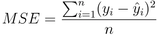
Mean Square Error/Quadratic Loss/L2 Loss (Regression Losses)
Mean square error is measured as the average of the squared difference between predictions and actual observations. It’s only concerned with the average magnitude of error irrespective of their direction. However, due to squaring, predictions that are far away from actual values are penalized heavily in comparison to less deviated predictions. Plus MSE has nice mathematical properties which make it easier to calculate gradients.
# Plain implementation

import numpy as np

y_hat = np.array([0.000, 0.166, 0.333])
y_true = np.array([0.000, 0.254, 0.998])

def rmse(predictions, targets):
    total_error = 0
    for yt, yp in zip(targets, predictions):
        total_error += (yt-yp)**2
    print("Total Squared Error:",total_error)
    mse = total_error/len(y_true)
    print("Mean Squared Error:",mse)
    return mse

print("d is: " + str(["%.8f" % elem for elem in y_hat]))
print("p is: " + str(["%.8f" % elem for elem in y_true]))

rmse_val = rmse(y_hat, y_true)
print("rms error is: " + str(rmse_val))
# Implementation using numpy

import numpy as np

y_hat = np.array([0.000, 0.166, 0.333])
y_true = np.array([0.000, 0.254, 0.998])

def rmse(predictions, targets):
    return np.mean(np.square(targets-predictions))

print("d is: " + str(["%.8f" % elem for elem in y_hat]))
print("p is: " + str(["%.8f" % elem for elem in y_true]))

rmse_val = rmse(y_hat, y_true)
print("rms error is: " + str(rmse_val))
Log Loss or Binary Cross Entropy
import numpy as np

y_predicted = np.array([[0.25,0.25,0.25,0.25],[0.01,0.01,0.01,0.96]])
y_true = np.array([[0,0,0,1],[0,0,0,1]])

def cross_entropy(predictions, targets, epsilon=1e-10):
    predictions = np.clip(predictions, epsilon, 1. - epsilon)
    N = predictions.shape[0]
    ce_loss = -np.sum(np.sum(targets * np.log(predictions + 1e-5)))/N
    return ce_loss
cross_entropy_loss = cross_entropy(predictions, targets)
print ("Cross entropy loss is: " + str(cross_entropy_loss))

# OR

def log_loss(predictions, targets, epsilon=1e-10):
    predicted_new = [max(i,epsilon) for i in predictions]
    predicted_new = [min(i,1-epsilon) for i in predicted_new]
    predicted_new = np.array(predicted_new)
    return -np.mean(targets*np.log(predicted_new)+(1-y_true)*np.log(1-predicted_new))
# Single Feature
import numpy as np
import matplotlib.pyplot as plt

%matplotlib inline

def gradient_descent(x, y, epochs = 10000, loss_thresold = 0.5, rate = 0.01):
    w1 = bias = 0
    n = len(x)
    plt.scatter(x, y, color='red', marker='+', linewidth='5')
    for i in range(epochs):
        y_predicted = (w1 * x)+ bias
        plt.plot(x, y_predicted, color='green')
        md = -(2/n)*sum(x*(y-y_predicted))
        yd = -(2/n)*sum(y-y_predicted)
        w1 = w1 - rate * md
        bias = bias - rate * yd
        print ("m {}, b {}, cost {} iteration {}".format(m_curr,b_curr,cost, i))

# Usage
x = np.array([1,2,3,4,5])
y = np.array([5,7,9,11,13])
gradient_descent(x, y, 500)

---

# Multiple Feature
def gradient_descent(x1, x2, y, epochs = 10000, loss_thresold = 0.5, rate = 0.01):
    w1 = w2 = bias = 1
    rate = 0.5
    n = len(x1)
    for i in range(epochs):
        weighted_sum = (w1 * x1) + (w2 * x2) + bias
        y_predicted = sigmoid_numpy(weighted_sum)
        loss = log_loss(y_predicted, y)

        w1d = (1/n)*np.dot(np.transpose(x1),(y_predicted-y))
        w2d = (1/n)*np.dot(np.transpose(x2),(y_predicted-y))

        bias_d = np.mean(y_predicted-y)
        w1 = w1 - rate * w1d
        w2 = w2 - rate * w2d
        bias = bias - rate * bias_d

        print (f'Epoch:{i}, w1:{w1}, w2:{w2}, bias:{bias}, loss:{loss}')

        if loss<=loss_thresold:
            break

    return w1, w2, bias

# Usage
gradient_descent(
    X_train_scaled['age'],
    X_train_scaled['affordibility'],
    y_train,
    1000,
    0.4631
)
# custom neural network class

class myNN:

    def __init__(self):
        self.w1 = 1
        self.w2 = 1
        self.bias = 0

    def sigmoid_numpy(self, X):
        import numpy as np;
        return 1/(1+np.exp(-X))

    def log_loss(self, y_true, y_predicted):
        import numpy as np;
        epsilon = 1e-15
        y_predicted_new = [max(i,epsilon) for i in y_predicted]
        y_predicted_new = [min(i,1-epsilon) for i in y_predicted_new]
        y_predicted_new = np.array(y_predicted_new)
        return -np.mean(y_true*np.log(y_predicted_new)+(1-y_true)*np.log(1-y_predicted_new))

    def fit(self, X, y, epochs, loss_thresold):
        self.w1, self.w2, self.bias = self.gradient_descent(X['age'],X['affordibility'],y, epochs, loss_thresold)
        print(f"Final weights and bias: w1: {self.w1}, w2: {self.w2}, bias: {self.bias}")

    def predict(self, X_test):
        weighted_sum = self.w1*X_test['age'] + self.w2*X_test['affordibility'] + self.bias
        return self.sigmoid_numpy(weighted_sum)

    def gradient_descent(self, age,affordability, y_true, epochs, loss_thresold):
        import numpy as np;
        w1 = w2 = 1
        bias = 0
        rate = 0.5
        n = len(age)
        for i in range(epochs):
            weighted_sum = w1 * age + w2 * affordability + bias
            y_predicted = self.sigmoid_numpy(weighted_sum)
            loss = self.log_loss.log_loss(y_true, y_predicted)

            w1d = (1/n)*np.dot(np.transpose(age),(y_predicted-y_true))
            w2d = (1/n)*np.dot(np.transpose(affordability),(y_predicted-y_true))

            bias_d = np.mean(y_predicted-y_true)
            w1 = w1 - rate * w1d
            w2 = w2 - rate * w2d
            bias = bias - rate * bias_d

            if i%50==0:
                print (f'Epoch:{i}, w1:{w1}, w2:{w2}, bias:{bias}, loss:{loss}')

            if loss<=loss_thresold:
                print (f'Epoch:{i}, w1:{w1}, w2:{w2}, bias:{bias}, loss:{loss}')
                break

        return w1, w2, bias


# Usage
customModel = myNN()
customModel.fit(X_train_scaled, y_train, epochs=8000, loss_thresold=0.4631)

# Usage
customModel = myNN()
customModel.fit(
        X_train_scaled,
        y_train,
        epochs=8000,
        loss_thresold=0.4631
)
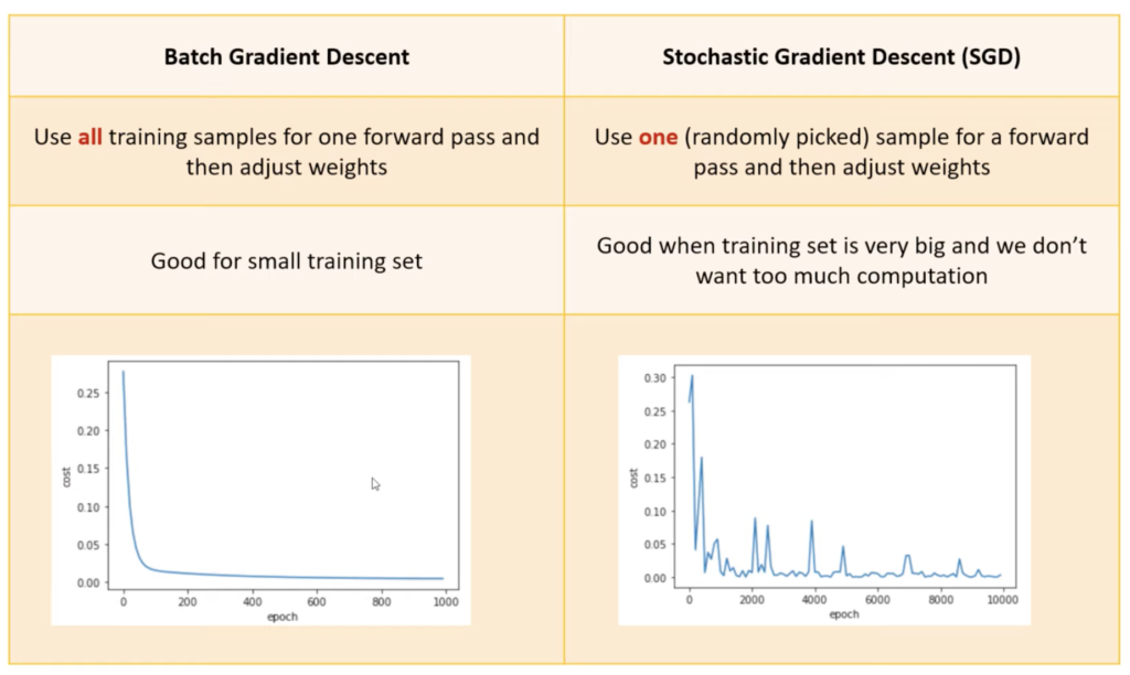
Batch Gradient Descent
def batch_gradient_descent(X, y_true, epochs, learning_rate = 0.01):

    number_of_features = X.shape[1]
    # numpy array with 1 row and columns equal to number of features. In
    # our case number_of_features = 2 (area, bedroom)
    w = np.ones(shape=(number_of_features))
    b = 0
    total_samples = X.shape[0] # number of rows in X

    cost_list = []
    epoch_list = []

    for i in range(epochs):
        y_predicted = np.dot(w, X.T) + b

        w_grad = -(2/total_samples)*(X.T.dot(y_true-y_predicted))
        b_grad = -(2/total_samples)*np.sum(y_true-y_predicted)

        w = w - learning_rate * w_grad
        b = b - learning_rate * b_grad

        cost = np.mean(np.square(y_true-y_predicted)) # MSE (Mean Squared Error)

        if i%10==0:
            cost_list.append(cost)
            epoch_list.append(i)

    return w, b, cost, cost_list, epoch_list

w, b, cost, cost_list, epoch_list = batch_gradient_descent(
    scaled_X,
    scaled_y.reshape(scaled_y.shape[0],),
    500
)
w, b, cost
Mini Batch Gradient Descent
def mini_batch_gradient_descent(X, y_true, epochs = 100, batch_size = 5, learning_rate = 0.01):

    number_of_features = X.shape[1]
    # numpy array with 1 row and columns equal to number of features. In
    # our case number_of_features = 3 (area, bedroom and age)
    w = np.ones(shape=(number_of_features))
    b = 0
    total_samples = X.shape[0] # number of rows in X

    if batch_size > total_samples: # In this case mini batch becomes same as batch gradient descent
        batch_size = total_samples

    cost_list = []
    epoch_list = []

    num_batches = int(total_samples/batch_size)

    for i in range(epochs):
        random_indices = np.random.permutation(total_samples)
        X_tmp = X[random_indices]
        y_tmp = y_true[random_indices]

        for j in range(0,total_samples,batch_size):
            Xj = X_tmp[j:j+batch_size]
            yj = y_tmp[j:j+batch_size]
            y_predicted = np.dot(w, Xj.T) + b

            w_grad = -(2/len(Xj))*(Xj.T.dot(yj-y_predicted))
            b_grad = -(2/len(Xj))*np.sum(yj-y_predicted)

            w = w - learning_rate * w_grad
            b = b - learning_rate * b_grad

            cost = np.mean(np.square(yj-y_predicted)) # MSE (Mean Squared Error)

        if i%10==0:
            cost_list.append(cost)
            epoch_list.append(i)

    return w, b, cost, cost_list, epoch_list

w, b, cost, cost_list, epoch_list = mini_batch_gradient_descent(
    scaled_X,
    scaled_y.reshape(scaled_y.shape[0],),
    epochs = 120,
    batch_size = 5
)
w, b, cost
Stochastic Gradient Descent
def stochastic_gradient_descent(X, y_true, epochs, learning_rate = 0.01):

    number_of_features = X.shape[1]
    # numpy array with 1 row and columns equal to number of features. In
    # our case number_of_features = 3 (area, bedroom and age)
    w = np.ones(shape=(number_of_features))
    b = 0
    total_samples = X.shape[0]

    cost_list = []
    epoch_list = []

    for i in range(epochs):
        random_index = random.randint(0,total_samples-1) # random index from total samples
        sample_x = X[random_index]
        sample_y = y_true[random_index]

        y_predicted = np.dot(w, sample_x.T) + b

        w_grad = -(2/total_samples)*(sample_x.T.dot(sample_y-y_predicted))
        b_grad = -(2/total_samples)*(sample_y-y_predicted)

        w = w - learning_rate * w_grad
        b = b - learning_rate * b_grad

        cost = np.square(sample_y-y_predicted)

        if i%100==0: # at every 100th iteration record the cost and epoch value
            cost_list.append(cost)
            epoch_list.append(i)

    return w, b, cost, cost_list, epoch_list

w_sgd, b_sgd, cost_sgd, cost_list_sgd, epoch_list_sgd = SGD(
    scaled_X,
    scaled_y.reshape(scaled_y.shape[0],),
    10000
)
w_sgd, b_sgd, cost_sgd